Parameter Sensitive Plan (PSP) Optimization, The Great Feature Coming with SQL Server 2022

The SQL Server 2022 is coming with fantastic new features. One of these features is Parameter Sensitive Plan Optimization.

The stored procedures are very useful and have a lot of advantages for the performance and the security.

You can see the differences between the ad hoc queries and the stored procedures below.

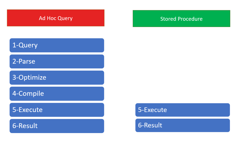
A query process completes with 6 steps in an ad hoc query. But it completes with 2 steps in stored procedures.

The first 4 steps run when the procedure first executed and then the execution plan stored in cache. The next time, we execute the stored procedure, we don’t need to run first 4 steps. Because it is still on cache. This situation is very useful and it increases the query performance.

But sometimes, it can cause a performance down. It depends on the first execution parameter.

The execution plan is created for the first parameter. And the execution plan contains the index for calling the stored procedure. If the next time, we call the stored procedure with a different parameter, need a different index, the cached plan chooses the wrong index and the query will be slower.

If we use the ad hoc query according to stored procedure, our query execution plan will choose the correct index. Because, when we call an ad hoc query, the execution plan is calculated for every query.

This is the problem.

The stored procedures, can be call with different parameters and every parameter may need different indexes, but the stored procedure has just one execution plan and one index.

And this is the solution!

The SQL Server 2022 has a new feature for this problem. We can store more than one execution plan for a stored procedure.

I will explain it with a dataset.

You can use the script below to create the sample database.

CREATE DATABASE SALESPSP
GO
USE SALESPSP 
GO 
CREATE TABLE ITEMS (ID INT IDENTITY(1,1) PRIMARY KEY,ITEMNAME VARCHAR(100),PRICE FLOAT)
DECLARE @I AS INT=1
DECLARE @PRICE AS FLOAT
DECLARE @ITEMNAME AS VARCHAR(100)
WHILE @I<=100
BEGIN
	 
	SET @PRICE =RAND()*10000
	SET @PRICE=ROUND(@PRICE,2)
	SET @ITEMNAME='ITEM'+REPLICATE('0',3-LEN(@I))+CONVERT(VARCHAR,@I)
	INSERT INTO ITEMS (ITEMNAME,PRICE) VALUES (@ITEMNAME,@PRICE )
SET @I=@I+1
END


SELECT * FROM ITEMS 


CREATE TABLE CUSTOMERS (ID INT IDENTITY(1,1) PRIMARY KEY,CUSTOMERNAME VARCHAR(100))
SET @I=1
DECLARE @CUSTOMERNAME AS VARCHAR(100)
WHILE @I<=100
BEGIN
	SET @CUSTOMERNAME='CUSTOMER'+REPLICATE('0',3-LEN(@I))+CONVERT(VARCHAR,@I)
	INSERT INTO CUSTOMERS (CUSTOMERNAME) VALUES (@CUSTOMERNAME)
SET @I=@I+1
END

CREATE TABLE SALES (ID INT IDENTITY(1,1) PRIMARY KEY,ITEMID INT,CUSTOMERID INT,DATE_ DATETIME,AMOUNT INT,PRICE FLOAT,TOTALPRICE FLOAT,DEFINITION_ BINARY(4000))
SET @I=0
DECLARE @ITEMID AS INT

DECLARE @AMOUNT AS INT
DECLARE @CUSTOMERID AS INT
DECLARE @DATE AS DATETIME 

WHILE @I<500000
BEGIN
	DECLARE @RAND AS FLOAT
	SET @RAND =RAND()

	IF @RAND<0.9
		SET @ITEMID =1
	ELSE 
		SET @ITEMID=(RAND()*99)+1

	SELECT @PRICE=PRICE FROM ITEMS WHERE ID=@ITEMID
	SET @CUSTOMERID=(RAND()*99)+1
	DECLARE @DAYCOUNT AS INT
	DECLARE @SECONDCOUNT AS INT
 
	SET @AMOUNT=(RAND()*19)+1
	SET @DAYCOUNT=RAND()*180
	SET @SECONDCOUNT=RAND()*24*60
	SET @DATE=DATEADD(DAY,@DAYCOUNT,GETDATE())
	SET @DATE=DATEADD(DAY,@SECONDCOUNT,@DATE )
	INSERT INTO SALES (ITEMID,CUSTOMERID,AMOUNT,PRICE,TOTALPRICE,DATE_)
	VALUES (@ITEMID,@CUSTOMERID,@AMOUNT,@PRICE,@PRICE*@AMOUNT,@DATE)
SET @I=@I+1
END
CREATE INDEX IX1 ON SALES (ITEMID)

We have 100 rows in the ITEMS table.

And we have 100 rows for the CUSTOMERS table.

Let’s look at the SALES table related with the ITEMS and the CUSTOMERS table.

We have 500.00 rows for the SALES table.

In this script, we are creating the rows by choosing a random ITEMID and random CUSTOMERID. But there is more probability to choose the 1 value for the ITEMID.

As we can see below, we have about 450.000 rows for the ITEMID=1 and 500-600 rows for the other ITEMIDs.

We have a primary key and clustered index contains the ID field and we have a nonclustered index in SALES table.

Let’s run the query.

SET STATISTICS IO ON 
SELECT ITEMID,SUM(AMOUNT) TOTALAMOUNT,
COUNT(*) ROWCOUNT_
FROM SALES 
WHERE ITEMID=20
GROUP BY ITEMID

Now, Let’s look at the query statistics and learn how many page did the query read.

The query reads 1709 pages and it’s equal that 1709×8/1024=13 MB.

Now let’s look at the execution plan.

The server optimizes itself by choosing the IX1 nonclustered index.

If we look at the IX1 index, wee see the ITEMID column. It is normal. I send a parameter to the query as ITEMID and query choose the index contains ITEMID.

Well, what happens if the system does not find the correct index, but performs a clustered index scan over the primary key? Let’s see this by doing index forcing.

SET STATISTICS IO ON 
SELECT ITEMID,SUM(AMOUNT) TOTALAMOUNT,
COUNT(*) ROWCOUNT_
FROM SALES WITH (INDEX=PK_SALES)
WHERE ITEMID=20
GROUP BY ITEMID

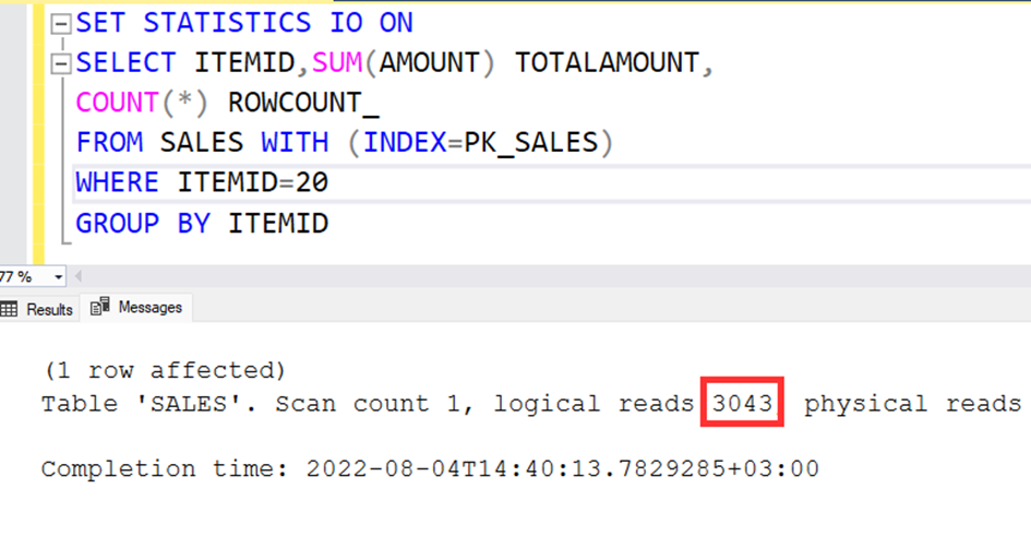
As you see, the read page count increased to two times. I think it’s not a big problem.

Well, Let’s call the query again with ITEMID=1.

SET STATISTICS IO ON 
SELECT ITEMID,SUM(AMOUNT) TOTALAMOUNT,
COUNT(*) ROWCOUNT_
FROM SALES  
WHERE ITEMID=1
GROUP BY ITEMID

The read page count is the same and 3043.

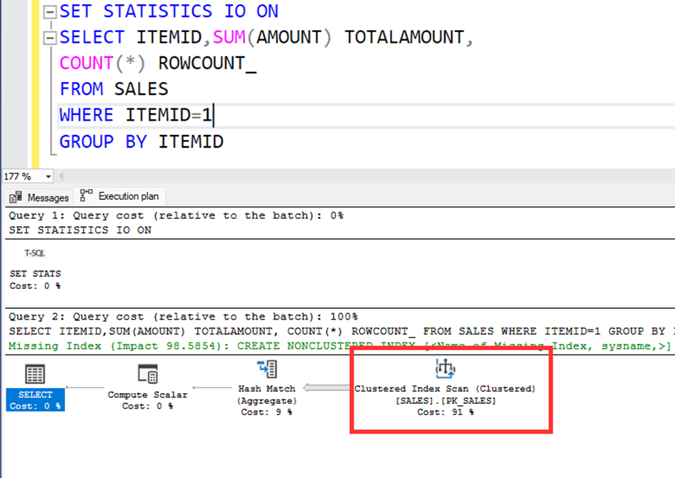
Let’s look at the execuion plan again.

According to execution plan, the system prefer the clustered index instead of nonclustered index. We know that, our parameter is ITEMID and we have an nonclustered index contains the ITEMID but the system choose the clustered index.

Because if we use the ITEMID=1, using the clustered index is more effective. Because there are 450.000 rows with the ITEMID=1.

Ok. Let’s force to use nonclustered index.

SET STATISTICS IO ON 
SELECT ITEMID,SUM(AMOUNT) TOTALAMOUNT,
COUNT(*) ROWCOUNT_
FROM SALES  WITH (INDEX=IX1)
WHERE ITEMID=1
GROUP BY ITEMID 

As we can see, the system reads so much.

The SQL Server can find the correct index by using the statistics and compile the correct plan. But we have a problem with the stored procedures. It is created the first time the Execution plan stored procedure run.

According to this rule, we have a risk. If the stored procedure will execute first with the parameter ITEMID=1, the procedure always use the clustered index for all the parameters. Or the first execution parameter’s frequency is less then, for example ITEMID=20, the execution plan will be create for the non clustered index.

In SQL Server 2022, we have a fantastic feature. The feature name is PSP (Parameter Sensitive Plan) Optimization. This feature allows to store mutiple execution plan for a stored procedure.

So we can use the stored procedures like the ad hoc queries.

Let’s try it. I create a stored procedure, named GETSALES_BY_ITEMID.

CREATE PROC [dbo].[GETSALES_BY_ITEMID]
@ITEMID AS INT
AS
BEGIN
	SELECT ITEMID,SUM(AMOUNT) TOTALAMOUNT,
	COUNT(*) ROWCOUNT_
	FROM SALES   
	WHERE ITEMID=@ITEMID 
	GROUP BY ITEMID 
END

Right click on the SALESPSP database, click properties and change the compatibility level to SQL Server 2019.

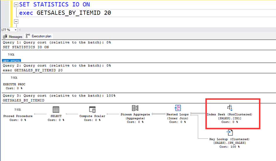
Now, run the procedure with ITEM=20 parameter.

Let’s look at the active execution plan.

Let’s look at the active execution plan.

Let’s call the procedure with the parameter ITEMID=1, again the system uses the IX1 nonclustred index. But it is not correct index. The clustered index is better fort he ITEM=1.

Let’s change the compatibility level to 2022 again.

When we call the procedure with ITEMID=1, the system uses the clustered index.

When we call the procedure with ITEMID=20, the system uses the non-clustered index.

Conclusion

The stored procedures are absolutely so important for the performance. But the stored procedures have only one execution plan for the different type of parameters. Because of this situation, the proc can choose the wrong index and it is not good for the performance.

In the SQL Server 2022, the stored procedures can store multiple execution plan and they can use the correct index, according to parameters. This is a really great feature. Thanks to SQL Server engineers.

I hope, you liked this article. See you on another article.

Why is correct normalization so important in database systems?

Hi,

In this article, i will talk about, choosing right data types and normalization on database tables.

The “Database” is a basic word.   It contains “Data” and “Base” words. So it means “The Base of Data”.

So, in databases, the correct definition of the data is more important than we guess.

We define the variable as “string” while we are coding.

But in database systems, there are a lot of data types to define a string data.

Unfortunately, we generally use nchar for string values and use bigint for integer values.

In this article, I will explain, how this situation causes a big problem.

Now, let’s imagine!

We have a task. Our task is to design a citizenship database table for a country.

For example my country Turkey. The population is now about 85 million. Let’s assume that with the people who died and the family tree, we have about 200 million people in our database.

Let’s design the table.

First of all, we have an ID column. The column has an auto-increment value and it is also the primary key of the table.

And the other columns are here.

ID                                        :Auto increment primary key value

CITIZENNUMBER            :11 digits unique citizen number

CITYID                                :The id number of the city where the citizen was born

TOWNID                            :The id number of the town where the citizen currently lives

DISTRICTID                       :The id number of the district where the citizen currently lives

NAMESURNAME             :The citizen’s name surname info

I think these are enough for an easy understanding of the subject.

Actually, this is enough to understand the results of wrong datatypes.

Let’s start from the ID column. We think firstly, this column will address about 200 million rows. So this is a very big value. So we think that we must use the “bigint” data type.

The next column is CITIZENNUMBER. This has 11 digits number and we choose the bigint again.

And the other columns are also integer values. Then let’s choose the bigint for all of them too.

Now let’s calculate it. A bigint value uses 8 Byte in the storage. Even we use just 1 or 0 for the value.
If we use the bigint value for all these columns, we need about 7.6 GB of space for the data.
We have just one table and just 5 numeric columns. I think it is too much.
Well, how can we reduce this huge space? Of course, by using the correct data types.
The bigint data types addresses values between  -2^63 and  +2^63.
Ok, do we need this huge gap for 200 million rows?
Of course not.
We have also an integer data type. The integer data type addresses values between -2^32 ile +2^32. It means between about -2 Billion and +2 Billion.
So, for the ID column, the integer data type is enough and better than the bigint. Because the integer data type uses just 4 Bytes. It is two times better than the bigint. And we know that the population will never be more than 2 Billion.

CITIZENNUMBER: This  column has 11 digits number. So an 11 digits value needs bigint.

CITYID: This column identifies the city Id from the Cities table. In Turkey country, we have just 81 cities and we know that it will always be less than 255. So we can use the TinyInt data types for the CityID column. The Tinyint datatype addresses the values between 1 and 255 and it uses just 1 Byte for a value.

TOWNIND: In Turkey, there are about 1.000 towns. So we can’t use the tinyint because it is not enough. But, we don’t want to use the integer. Because 2 Billion is so much for a value between 1 and 1000. There is another data type Smallint. The Smallint  data type addresses the values between -32.000  and +32.000. So the Smallint is suitable for the TOWNID column.

DISTRICTID:
Turkey has about 55.000 districts. So I can’t use the Tinyint and Smallint. But the Bigint is so much for this type of value. Then the Integer is good for this column.

Now, let’s calculate again. We can see the total space. It is about 3.54 GB. It is about two times better than the first design.

Let’s look at a string column. NameSurname.
In the country, there are citizens from all over the World. So if we define a max character limit, we have to calculate the max character limit of the names from all over the World.
For example, I know that the Spanish people have the longest names. Because they give names to their children as father’s, grand father’s, grand grand father’s names. 😊
For example
“pablo diego josé francisco de paula juan nepomuceno maría de los remedios cipriano de la santísima trinidad ruiz y Picasso”
We just say “Pablo Picasso” 😊
If we want to keep this name-surname information on the database, we have to use 250 digits for namesurname.
This data type is a string. But in database systems, there are so many data types used for string values.
Char, nchar, varchar,nvarchar etc.
Let’s explain the differences between these types with a basic example.
Let’s create a table with the columns below and save it as TEST.
ID:Int
NAME1:char(50)
NAME2:nchar(50)
NAME3:varchar(50)
NAME4:nvarchar(50)

Let’s insert my name, “ÖMER” to the table.

Let’s query the table.

I copy the value from the NAME1 column and paste it into an empty place.

Did you see where the cursor is blinking?

It is blinking far from the end of the string value. The name value “ÖMER” has 4 digits length but the cursor is blinking at 50 digits length. It means, the char(50) uses 50 digits for any value less or equal to 50 digits. It is a very big disadvantage. Think! We have a lot of short names, for example, Jhon, Marry, May, etc. Their average length is just  4 characters and it is a really huge waste.

Let’s investigate the NAME2 column. Copy the NAME2 column and paste it into the text area.

The situation is the same. The cursor is blinking at the end of the 50th character. So, we can say that char and nchar may be the same.

Now let’s look at NAME3 and NAME4 columns. NAME3 is varchar and NAME4 is Nvarchar. Copy the NAME3 and paste into the free text space.

Can you see where the cursor is blinking? The cursor is blinking at the end of the string. The length of the string is 4 digits and the cursor is blinking here. So we can understand that the varchar data type uses space as the string value’s length not max length.

According to this scenario, the char data type uses 50 digits and varchar uses just 4 digits. I think it’s really better than the char or nchar.

We can see that the Nvarchar is the same as the varchar. We don’t know what the “N” means on Nchar or Nvarchar does yet.

The “N” character symbolizes Unicode support. Unicode means the international characters.

Let me show you with an example to understand what Unicode support is.

I use google translate and translate a word to into Chinese. The first word that comes to my mind is book. In Chinese, “书” word means “book”. So I copy this word and paste it into the table.

And I select the data from the table below.

You can see that in the NAME1 and NAME3 columns we can’t see the Chinese character. These columns are both char and varchar and do not support the Unicode characters. It is very easy to understand. Char and Varchar data types use 1 Byte for each letter or character. 1 Byte means 0-255 different numbers. For example, in alphabet, there are 26 characters. So we have 26 lowercase and 26 uppercase letters, 10 numbers, and a lot of punctuations. 255 is enough to address all these letters. But think about the Japanese alphabet. The Japanese alphabet has about 2.000 letters. So 1 byte is not enough for all these characters. We need more. Maybe 2 Bytes can be suitable for us. 2 bytes addresses about 32.000 different letters. Nchar and Nvarchar uses 2 bytes for a letter and can show the Unicode characters.

Let’s turn the scenario again. We have 200 million rows that include namesurname column with max 250  digits and with Unicode support.

Then we have to use nchar(250) or nvarchar(250).

Using nchar(250) is a wrong stuation. Because 250 is just a limit but we arrange 250×2=500 Bytes for all namesurnames.

Using nvarchar (250) is the best choice. Because it supports Unicode characters and also uses space as the namesurname’s length.

Let’s calculate again

As you see, in the wrong design, we use about 100 GB. But in the correct design, we use just 11 GB. It is 10 times smaller than the first one.

We are talking about just one table and just 6 columns. And even in this situation, we can see a huge difference.

In database systems, we have a lot of tables with a lot of columns.

In this article, we talked about the normalization and importance of choosing the right data type.

We talked about the size of the data. You can think that it is only about the size on the disk and you can ignore all these calculations in your mind. You can say “It is all about the money. I can use bigger storage.”  But it is a wrong approach. Because it is not about just the storage. Because SQL Server works on memory and uses the CPU.

If the data type is bigint, You use 8 Byte space on your ram for the for example, 15 number.

If the data type is tinyint, You use 1 Byte space on your ram for the 15 number.

And also if you use bigint, you can use your CPU 8 times more.

As a result,

The Normalization and the knowing to use the right data types are more important than we guess.

See you again in the next article.

2021 nasıl geçti?

Acısıyla, tatlısıyla bir yılı daha geride bıraktık.Zor ve yorucu bir covid tedavisi ile geçen pandemi dönemini saymazsak 2021 tam da istediğim gibi çalışarak, paylaşarak ve üreterek geçti.2022 yılının ise yeni şeyler öğrendiğim, daha çok ürettiğim ve tabi ki daha çok paylaştığım bir yıl olmasını diliyorum.2021 yılında etrafımda çoğunlukla beni motive eden, beni mutlu eden insanlar yer almış. 2021’in benim için keyifli ve güzel olan bazı anılarını bu videoda toparladım.2022 yılının hepimiz için sağlık, mutluluk, huzur ve barış getirmesini dilerim.Benim 2021’imin nasıl geçtiğini merak edenler için,Buyursunlar. 👇

SQL Server’da hangi db ler kullanılıyor? Hangisi kullanılmıyor?

Merhaba,

SQL Server’da bir çok database iniz var. Hangisi aktif kullanılıyor, hangisi kullanılmıyor görmek istiyorsunuz. En son ne zaman erişildiğini görmek için aşağıdaki scripti görebilirsiniz.

CREATE TABLE #T (dbName varchar(100),last_user_seek datetime,last_user_scan datetime,last_user_lookup datetime,last_user_update datetime)
declare @dbId as int
declare @dbname as varchar(100)
declare crs cursor for select dbid,name from sysdatabases 
open crs
fetch next from crs into @dbId,@dbname
while @@FETCH_STATUS=0
begin
Insert Into #T 
Select @dbname,
last_user_seek = MAX(last_user_seek),
last_user_scan = MAX(last_user_scan),
last_user_lookup = MAX(last_user_lookup),
last_user_update = MAX(last_user_update)
From
sys.dm_db_index_usage_stats
WHERE
database_id=@dbId

fetch next from crs into @dbId,@dbname
end 
close crs
deallocate crs 
 
select * from #t 
drop table  #t 

SQL Server Üzerinde TSQL ile RFM Analizi, Müşteri Segmentasyonu

Merhaba,

Bu yazıda veri bilimi konusunda sıklıkla yapılan çalışmalardan RFM konusunun SQL Server üzerinde T-SQL kodları yazarak nasıl yapılacağını uygulamalı şekilde anlatacağım.

Konuyu bilmeyenler için RFM Analizi ne demek biraz bahsedelim.

RFM nedir?

Recency, Frequency, Monetary kelimelerinin baş harflerinden oluşup, bu üç metriğin hesaplanmasından sonra birleştirilmesiyle meydana gelen bir skordur. Müşterilerin mevcut durumunun analiz edilip, bu skorlara göre segmentlere ayrılmasına yardımcı olur.

Recency: Müşterinin ne kadardır websitesinden/mağazadan hizmet aldığı, ne zamandır bize üye olduğu gibi bilgileri verir. Hesaplanması genellikle, bugünden son üyelik tarihi/son sipariş tarihinin çıkartılmasıyla elde edilir.

Frequency: Müşterinin ne sıklıkla alışveriş yaptığını, ne sıklıkla siteye giriş yaptığını gösteren metriktir. Genellikle sipariş numarası/sipariş kodunun saydırılmasıyla sonuç verir.

Monetary: Müşterinin harcamalarının toplamıdır. E-ticaret sitesine getirdiği ciro, aldığı hizmetler sonrası toplanan getiri olarak da tanımlanabilir. Ciro tanımı ne ise, müşteri bazında hayatı boyunca yapılan harcamalar toplanarak hesaplanır.

Bu metrikler belirlendikten sonra, metrik bazında müşteri verisi 5 eşit parçaya ayrılır. Sonrasında bu rakamlar bir araya getirilerek bir RFM skoru atanır.

Kaynak: https://www.veribilimiokulu.com/rfm-analizi-ile-musteri-segmentasyonu/

RFM analizi bir satış veriseti üzerinde çalışarak elde edilir ve yapılan çalışma sonucunda bir müşteri sınıflandırma işlemi gerçekleştirilir.

Elde etmek istediğimiz tablo aşağıdaki gibidir.

Burada alanların açıklamaları aşağıdaki gibidir.

CustomerID:Sınıflandırılamak istenen müşterinin ID’sidir. Burada müşteri kodu, müşteri adı gibi bilgiler de olabilir.

LastInvoiceDate:Müşterinin son alışveriş yaptığı tarih ve zaman bilgisini tutar. Bu bilgi bizim Recency değerimizi hesaplamak için kullanacağımız bir alandır.

Recency: Müşterinin en son ne zaman alışveriş yaptığı bilgisinin bir metriğidir. Bugün-Son alışveriş tarihi olarak hesaplanır.

Frequency: Müşterinin ne sıklıkta alışveriş yaptığı bilgisidir. Burada fatura numarası ya da sipariş numarası gibi alanlar distinct olarak sayılarak bulunur.

Monetary: Müşterinin harcamalarının toplamıdır. Yani toplamda bir müşteri parasal olarak ne kadarlık alışveriş yapıyor onun karşılığıdır.

Recency_Scale: Elde edilen Recency değerinin 1-5 arasına sıkıştırılmış halidir. Daha açıklayıcı anlatmak gerekirse, diyelim 100 satır kaydımız var.

100/5=20

Demek ki tüm veriyi Receny değerine göre sıralar isek

Sıralamada

1-20 arası=1

21-40 arası=2

41-60 arası=3

61-80 arası=4

81-100 arası=5 olacak şekilde bir yeniden boyutlandırma (Scale) işlemi yapılmaktadır.

Frequency _Scale: Elde edilen Frequency değerinin 1-5 arasına sıkıştırılmış halidir.

Monetary _Scale: Elde edilen Monetary değerinin 1-5 arasına sıkıştırılmış halidir.

Segment: Elde edilen Recency_Scale, Frequency _Scale, Monetary _Scale değerlerine göre belli bir formül ile müşterinin sınıflandırılmasıdır. Bu sınıflandırmada müşteriler Need_Attention, Cant_Loose,At_Risk,Potential_Loyalists, Loyal_Customers, About_to_Sleep,Hibernating,New_Customers, Promising, Champions

Sınıflarından birine göre sınıflandırılır.

Hadi şimdi işe koyulalım ve RFM analizi için önce veri setimizi indirelim.

Verisetimiz https://archive.ics.uci.edu/ml/machine-learning-databases/00502/online_retail_II.xlsx adresindeki online_retail_II.xlsx isminde bir excel dosyası.

Bu dosyayı indirelim.

Görüldüğü gibi dosyamız bu şekilde bir görünüme sahip.

Dosyada 2009-2010 ve 2010-2011 yılına ait satış verileri bulunmakta. Biz uygulamamızda bu iki veriden birini seçip çalışacağız. İstenirse bu iki veri birleştirilebilir. Biz şimdilik Year 2010-2011 verilerini dikkate alalım.

Bu sayfaya baktığımızda 540.457 satırlık bir verinin olduğunu görüyoruz. Tabi burada bir müşteriye ait birden fazla fatura var ve bir faturanın altında da birden fazla ürün satırı var. O yüzden satır sayısı bu kadar fazla.

Şimdi kolonlardan biraz bahsedelim.

Invoice: Fatura numarası

StockCode: Satılan ürünün kodu

Description: Satılan ürünün adı

Quantity: Ürün adedi

InvoiceDate: Fatura tarihi

Price: Ürün birim fiyatı

Customer Id: Müşteri numarası

Country: Müşterinin ülkesi

Şimdi bu excel dosyamızı da gördüğümüze göre artık SQL Server platformuna geçme vakti. Malum yazımızın konusu RFM analizini MSSQL üzerinde gerçekleştirme.

İlk iş bu excel datasını SQL Server’a aktarmak.

Bunun için SQL Server üzerinde RFM isimli bir veritabanı oluşturalım.

Bunun için aşağıdaki gibi New Database diyerek yeni bir database oluşturabiliriz.

RFM isimli database imiz oluştu.

Şimdi bu database e excel dosyasındaki veriyi import edeceğiz. Bunun için database üzerinde sağ tıklayarak Task>Import Data diyoruz.

Next butonuna bastığımızda aşağıdaki hatayı alıyorsanız merak etmeyin çözümü var. Hata almıyorsanız bu kısmı okumasanız da olur.

Bu hatada Microsoft.Ace.Oledb.12.0 provider hatasını görüyoruz. Bu hatayı gidermek için Microsoft Access Database Engine’i bilgisayarınıza yüklemeniz gerekiyor. Bunun için aşağıdaki linki kullanabilirsiniz.

https://www.microsoft.com/en-us/download/confirmation.aspx?id=13255

Kurulumu next diyerek default ayarları ile yapabilirsiniz.

Ve kurulum tamamlandı.

Şimdi tekrardan Excel dosyamızı import ediyoruz. Import/Export wizard da kaynak olarak Excel dosyamızı göstermiştik. Hedef olarak ise SQL Server’ı göstereceğiz.

Bağlanacağımız SQL Server’ı seçiyor ve kullanıcı bilgilerini giriyoruz. Benim kullandığım SQL Server kendi makinem olduğu için server name kısmına localhost yazıyor, kullanıcı bilgilerine de Windows authentication’ı işaretliyoruz. Siz de kendi bağlandığınız SQL Server bilgilerini girebilirsiniz.

Copy data from one or more tables or views seçeneğini seçiyoruz.

Next dediğimizde karşımıza aşağıdaki ekran geliyor. Source kısmında Excel dosyasındaki sheet adı, Destination kısmında ise SQL Server’da oluşturacağımız tablonun adı geliyor. Burayı elle değiştirebiliyoruz. 2010-211 yılları arasındaki veriyi kullanmayı tercih ediyoruz.

SQL Server’a aktaracağımız tablonun adını ONLINERETAIL_2010 olarak değiştiriyoruz.

Burada Next deyip devam edebiliriz ancak Edit Mappings butonuna basıp yeni oluşan tablonun alanlarını ve veri tiplerini de görebiliriz. Edit Mappings butonuna basında biraz bekleyebilirsiniz. Zira 540.000 satır excel dosyasını okurken ki bekletme bu. Bilgisayar dondu diye panik yapmayın. Biraz beklediğinizde aşağıdaki ekranı göreceksiniz. Tablomuzun alanları ve veri tipleri. OK deyip geçebiliriz.

Next dediğimizde Run Immediately seçeneğini işaretliyoruz ve tekrar Next diyoruz.

Finish diyoruz ve satırlarımızın aktarılmasını bekliyoruz.

Import işlemi tamamlandı.

Şimdi kontrol edelim.

Artık excel dosyamız veritabanımızda. Buraya kadar ki işlemlerde hata yaşadıysanız. Çalıştığımız veritabanını buradaki linkten indirebilirsiniz.

https://1drv.ms/u/s!AoTudRti4cT8jLEZ3ShT6I2BtteHBw?e=3X4xfl

Artık verilerimizi aktardığımıza göre şimdi RFM analizi işlemlerine başlayabiliriz.

Yazımızın ilk başında RFM analizi sonucunda aşağıdaki gibi bir tablo elde etmek istediğimizden bahsetmiştik.

Bu tabloyu elde etmek için yapılan en büyük hatalardan biri karmaşık SQL cümleleri yazarak tek seferde bu tabloyu elde etmeye çalışmak. Şayet SQL bilginiz de çok iyi değilse geçmiş olsun. SQL ile RFM çalışmanız burada son bulacak büyük ihtimalle.

Şimdi daha basit düşünelim. Sonuçta bir excel tablomuz var. Burada tekrar etmeyen CustomerID ler var ve bu CustomerID lere göre hesaplanan bir takım sütunlar var. O zaman aynı bu mantıkta düşünelim ve bu mantıkta bir tablo oluşturup içine önce CustomerId’leri tekrar etmeyecek şekilde dolduralım. Sonra sırayla diğer alanları hesaplayarak gidelim.

İlk iş bu formatta bir SQL tablosu oluşturmak.

Ekteki gibi bir tablo oluşturuyoruz.

Şimdi her seferinde aynı işlemi yapacağımız için önce tablomuzun içini boşaltacak kodumuzu yazalım.

TRUNCATE TABLE RFM

Sonra tablomuzun için tekrar etmeyecek şekilde CustomerID’ler ile dolduralım. Bunun için kullanacağımız komut,

INSERT INTO RFM (CUSTOMERID)
SELECT DISTINCT [Customer ID] FROM ONLINERETAIL_2010

Burada excelden aktarırken Customer ID kolonunda boşluk olduğu için Customer ID yazarken köşeli parantezler içinde yazıyoruz.

4373 kayıt eklendi dedi. Şimdi tablomuzu kontrol edelim.

Şu anda içinde sadece CustomerId olan diğer alanları null olan 4373 satır kaydımız var.

Şimdi sırayla diğer alanları hesaplayalım. İlk hesaplayacağımız alan LastInvoiceDate. Yani müşterinin yaptığı son satınalma zamanının bulunması. Bu değeri bulacağız ki Recency değeri bu tarih ile şimdiki zamanın farkı üzerinden çıkarılacak ve buna göre bulunacak.

Bu işlem için basit bir update cümlesi kullanabiliriz. Aşağıdaki sorgu her bir müşterinin ONLINERETAIL tablosunda son alışveriş yaptığı zamanı bulup update edecektir.

UPDATE RFM SET LastInvoiceDate=(SELECT MAX(InvoiceDate) 
FROM ONLINERETAIL_2010 where [Customer ID]=RFM.CustomerID)

Update ettik. Şimdi de sonuca bakalım. Artık LastInvoiceDate alanımız da güncellenmiş durumda.

Bir sonraki adım Recency değerinin bulunması. Bunun için şimdiki zamandan son alışveriş zamanını çıkarmamız ve tablomuzu güncellememiz gerekiyor. Tıpkı bir excel dosyasında satır satır formül çalıştırır gibi sorgu ile satır satır güncelleme yapacağız.

SQL Server’da iki tarih arasındaki farkı alan komut DateDiff komutu. Burada datediff komutu içine üç parametre alır.

1-Farkı ne türünden alacaksın? Gün, Ay, Yıl…

2-Başlangıç zamanı (LastInvoiceDate)

3-Bitiş zamanı (Şimdiki zaman. Fakat bizim veri setimiz 2011 yılında geçtiği için son zamanı 31.12.2011 olarak alabiliriz.

Şimdi update cümlemizi çalıştıralım.

UPDATE RFM SET Recency=DATEDIFF(DAY,LastInvoiceDate,'20111231')

Sonuca bakalım.

Görüldüğü gibi Recency değerini hesaplatmış durumdayız. Sırada Frequency var. Şimdi de onu aşağıdaki sorgu ile bulalım. Frequency bir kişinin ne sıklıkta alışveriş yaptığı bilgisi idi. Yani fatura numaralarını tekil olarak saydırırsak bu değeri bulabiliriz.

UPDATE RFM SET Frequency=(SELECT COUNT(Distinct Invoice) FROM ONLINERETAIL_2010 where CustomerID=RFM.CustomerID)

Şimdi sonuca tekrar bakalım. Görüldüğü gibi Frequency değerimizi de hesapladık.

Sırada Monatery değerimiz var. Yani bir müşterinin yapmış olduğu toplam alışverişlerin parasal değeri. Bunu da aşağıdaki sql cümlesi ile bulabiliriz. Burada her bir müşteri için birim fiyat ile miktarı çarptırıyoruz.

UPDATE RFM SET Monatery=(SELECT sum(Price*Quantity)  FROM ONLINERETAIL_2010 where CustomerID=RFM.CustomerID)

Sonuçlara bakalım. Görüldüğü gibi Monatery değeri de hesaplanmış oldu.

Artık bu aşamadan sonra R,F ve M değerleri için scale değerlerini hesaplamaya sıra geldi. Bunun için tüm değerleri istenilen kolona göre sıralayıp sıra numarasına göre 1-5 arası değerlendirmeye tabi tutmamız gerekiyor. Bunun için kullanacağımız komut ise Rank komutu.

Kullanımı ise aşağıdaki gibi. Kullanımı karışık gelirse copy-paste yapmanız yeterli.

UPDATE RFM SET Recency_Scale= 
(
 select RANK from
 (
SELECT  *,
       NTILE(5) OVER(
       ORDER BY Recency desc) Rank
FROM RFM
) t where  CUSTOMERID=RFM. CUSTOMERID)

Sonuçlara baktığımızda artık Recency_Scale değerini de hesaplamış durumdayız.

Sırada Frequency_Scale var. Onun için de aşağıdaki komutu kullanıyoruz.

update RFM SET Frequency_Scale= 
(
 select RANK from
 (
SELECT  *,
       NTILE(5) OVER(
       ORDER BY Frequency) Rank
FROM rfm 
) T where  CUSTOMERID=RFM. CUSTOMERID)

Sonuca bakalım. Görüldüğü gibi Frequency_Scale’ da hesaplanmış durumda.

Ve son olarak Monatey_Scale değeri. Onu da aşağıdaki gibi hesaplıyoruz.

update RFM SET Monatery_Scale= 
(
 select RANK from
 (
SELECT  *,
       NTILE(5) OVER(
       ORDER BY Monatery) Rank
FROM rfm 
) t where  CustomerID=RFM.CustomerID)

Sonuçlara bakalım. Görüldüğü gibi Monatery_Scale’da hesaplandı.

Son olarak artık tüm değişkenlerimiz hesaplandığına göre geriye bir tek sınıflandırma etiketi kaldı. Onun sorgusu hazır durumda. Aşağıdaki sorguya göre sınıflandırmalar yapılabilir.

UPDATE RFM SET Segment ='Hibernating' 
WHERE Recency_Scale LIKE  '[1-2]%' AND Frequency_Scale LIKE '[1-2]%'  
UPDATE RFM SET Segment ='At_Risk' 
WHERE Recency_Scale LIKE  '[1-2]%' AND Frequency_Scale LIKE '[3-4]%'  
UPDATE RFM SET Segment ='Cant_Loose' 
WHERE Recency_Scale LIKE  '[1-2]%' AND Frequency_Scale LIKE '[5]%'  
UPDATE RFM SET Segment ='About_to_Sleep' 
WHERE Recency_Scale LIKE  '[3]%' AND Frequency_Scale LIKE '[1-2]%'  
UPDATE RFM SET Segment ='Need_Attention' 
WHERE Recency_Scale LIKE  '[3]%' AND Frequency_Scale LIKE '[3]%' 
UPDATE RFM SET Segment ='Loyal_Customers' 
WHERE Recency_Scale LIKE  '[3-4]%' AND Frequency_Scale LIKE '[4-5]%' 

UPDATE RFM SET Segment ='Promising' 
WHERE Recency_Scale LIKE  '[4]%' AND Frequency_Scale LIKE '[1]%' 
UPDATE RFM SET Segment ='New_Customers' 
WHERE Recency_Scale LIKE  '[5]%' AND Frequency_Scale LIKE '[1]%' 
UPDATE RFM SET Segment ='Potential_Loyalists' 
WHERE Recency_Scale LIKE  '[4-5]%' AND Frequency_Scale LIKE '[2-3]%' 
UPDATE RFM SET Segment ='Champions' 
WHERE Recency_Scale LIKE  '[5]%' AND Frequency_Scale LIKE '[4-5]%'

Sonuçlara bakalım.

Artık tüm müşterilerimizi sınıflandırmış durumdayız. Hatta hangi sınıftan kaç müşteri olduğuna da bakalım.

Vee işlem tamam.

Bu yazımızda SQL Server üzerinde sadece TSQL kodları kullanarak RFM Analizi çalışması yaptık. Çalışmada Online Retail datasını kullandık. Aşağıdaki kodu kullanarak OnlineRetail datasını aktardıktan sonraki tüm RFM hesaplama işlemlerini tek seferde yapabilirsiniz.

Buraya kadar sabırla okuduğunuz için çok teşekkür ederim.

Sağlıcakla…

SQL Databaselerinin aylık ne kadar büyüdüğünü gösteren sorgu

Merhaba,

İleriye yönelik sistem kaynak planlaması yaparken verilerinizin ne kadar büyüdüğünü görmek önemlidir. Aşağıdaki script sql backupları üzerinden databaselerinizin aylık ne kadar büyüdüğünü göstermektedir. Güzel ve kullanışlı bir script olduğu için paylaşmak istedim. Kaynak:https://www.mssqltips.com/

SELECT DATABASE_NAME,YEAR(backup_start_date) YEAR_ ,MONTH(backup_start_date) MONTH_ ,
MIN(BackupSize) FIRSTSIZE_MB,max(BackupSize) LASTSIZE_MB,max(BackupSize)-MIN(BackupSize) AS GROW_MB,
ROUND((max(BackupSize)-MIN(BackupSize))/CONVERT(FLOAT,MIN(BackupSize))*100,2)  AS PERCENT_
 FROM
(
SELECT
	s.database_name
,	s.backup_start_date
,	COUNT(*) OVER ( PARTITION BY s.database_name ) AS SampleSize
,	CAST( ( s.backup_size / 1024 / 1024 ) AS INT ) AS BackupSize
,	CAST( ( LAG(s.backup_size ) 
		OVER ( PARTITION BY s.database_name ORDER BY s.backup_start_date ) / 1024 / 1024 ) AS INT ) AS Previous_Backup_Size
FROM
	msdb..backupset s
WHERE
	s.type = 'D' --full backup
	and s.database_name='<dbname>'
) T GROUP BY DATABASE_NAME,MONTH(backup_start_date),YEAR(backup_start_date) 

Kaggle’da Paylaştığım Yeni Veriseti. TMDB Sitesi Verileri

Hey, Veri avcıları!
Sizin için güzel bir sürprizim var. Kaggle’a yeni dataset yükledim. 18 tablodan oluşan TMDB sitesinin film database’i. İçinde neler yok ki?
160.000+ Film
480.000+ Aktör
1400.000+ Film ekibi
17.000+ Anahtar kelime
48.000+ Yapımcı firma
1.5M+ Film Önerisi
900+ Meslek grubu.
Hem de ilişkisel şekilde. DB normalde MSSQL formatında ama herkes kullanabilsin diye excel formatına çevirip attım tüm tabloları. Beğeneceğinizi ümit ediyorum.
Bu arada Kaggle’da “Dataset Expert” olmuşum. Bir sonraki adım “Dataset Master” olmak.

https://www.kaggle.com/omercolakoglu/tmdb-website-movie-database/

Murat Yücedağ ile Veri Üzerine Sohbet

Nedir bu “Veri ile Konuşma” felsefesi? Kurumsal plaza dilinin özenti bir cümlesi mi yoksa gerçekten sokaktaki insanın anlayacağı ve işine yarayacağı bir kavram mı?
Hadi bu veri ile konuşma kavramının biraz daha ötesine gidelim.

1.Veri ile konuşma
2.Veri’yi konuşma
3.Veri’nin konuşması

3.sü en sevdiğim. Sevgili Murat Goce abinin Bilişim Zirvesi 2019’da kullandığı ve çok hoşuma giden “Data Talks” sloganı.
Evet. Bizler veri ile konuşma mertebesindeyken dünya veriyi konuşturuyor.

Hepsi ve daha fazlasını ziyadesiyle bulacağınız bir sohbet yaptık sevgili Murat Yücedağ ile. Evde geçirilen pazar günü için güzel bir alternatif olabilir.
Tanıtım faslını atlamak isteyenler doğrudan 00:09:40’dan başlayabilirler.
İyi seyirler.

Üsküdar Üniversitesi, Büyük Veri Analitiği Webcast

 Üsküdar Üniversitesi Yapay Zekâ ve Bilgi Güvenliği Kulübü ile birlikte Büyük Veri Analitiği ve Veri Görselleştirme konusunda canlı bir atölye yaptık. Yaklaşık 3 saat süren etkinlikte,
-Veri kavramı
-İş Zekası
-Veri Görselleştirme
-Veri Analitiği
kavramları üzerinde konuştuk.
Sonrasında
-17.000 müşteri
-28.000 ürün
-80 şube
-Yarım milyon satış verisi içeren bir verinin dashboardlarını oluşturduk.

Devexpress Dashboard ve Visual Studio kullanarak 2 saatten daha az bir sürede 4 tane analitik dashboard tasarladık ve son kullanıcının görebileceği hale getirdik.
Ayrıca gecenin sürprizi olarak aramızda olan özel sektör IT yöneticileri ve Türkiye’de İş Zekası yazılımı geliştiren firma sahibi abilerimizin öğrenci arkadaşlar ile yaptığı sektörel sohbetler oldu.
Bu arada öğrenci kardeşlerimiz için de staj fırsatı yakaladık.
Velhasıl, güzel, dolu dolu, keyifli bir etkinlikti.
Ümit ediyorum ki genç kardeşlerimin veri ve veri analitiği konusuna bakış açıları biraz değişmiştir.
Etkinliğin youtube kaydına buradan ulaşabilirsiniz.
Emeği geçen herkese teşekkür ederim.